Tweaks to the projected costs and benefits of prospective regulations or programs can be a great way to encourage domination of resources and society by the state. Of course, public policy ideas will never receive serious consideration unless their “expected” benefits exceed costs. It’s therefore critical that the validity of cost and benefit estimates — to say nothing of their objectivity — are always subject to careful review. By no means does that ensure that the projections are reasonable, however.
Traditionally less scrutinized is the rate at which the future costs and benefits of a program or regulation are discounted into present value terms. The discount rate can have a tremendous impact on the comparison of costs and benefits when their timing differs significantly, which is usually the case.
Intertemporal Tradeoffs
People generally aren’t willing to forsake present pleasure without at least a decentprospect of future gain. Thus, we observe that the deferral of $1 of consumption today generally brings a reward of more than $1 of future consumption. That’s made possible by the existence of productive opportunities for the use of resources. These opportunities, and the freedom to exploit them, allow a favorable tradeoff at which we transform resources across time for the benefit of both our older selves and our progeny. The interaction of savers and investors in such opportunities results in an equilibrium interest rate balancing the supply and demand for saving.
We can restate the tradeoff to demonstrate the logic of discounting. That is, the promise of $1 in the future induces the voluntary deferral of less than $1 of consumption today. To arrive at the amount of the deferral, the promised $1 in the future is discounted at the consumer’s rate of time preference. The promised $1 must cover the initial deferral of consumption plus the consumer’s perceived opportunity cost of lost consumption in the present, or else the “trade” won’t happen.
Discounting practices are broadly embedded in the economy. They provide a rational basis of evaluating inter-temporal tradeoffs. The calculation of net present values (NPVs) and internal rates of return (the discount rate at which NPV = 0) are standard practices for capital budgeting decisions in the private sector. Public-sector cost-benefit analysis often makes use of discounting methodology as well, which is unequivocally good as long as the process is not rigged.
Government Discounting
The Office of Management and Budget (OMB) provides guidance to federal agencies on matters like cost-benefit analysis. As part of a recent proposal that was prompted by executive orders on “Modernizing Regulatory Review” from the Biden Administration, the OMB has recommended revisions to a 2003 Circular entitled “Regulatory Analysis”. A major aspect of the proposal is a downward adjustment to recommended discount rates, largely dressed up as an update for “changes in market conditions”.
Since 2003, the OMB’s guidance on discount rates called for use of a historical average rate on 10-year government bonds. Before averaging, the rate was converted to a “real rate” in each period by subtracting the rate of increase in the Consumer Price Index (CPI). The baseline discount rate of 3% was taken from the average of that real rate over the 30 years ending in 2002. There has been an alternative discount rate of 7% under the existing guidance intended as a nod to the private costs of capital, but it’s not clear how seriously agencies took this higher value.
The new proposal seeks to update the calculation of recommended discount rates by using more recent data on Treasury rates and inflation. One aspect of the proposal is to utilize the rate on 10-year inflation-indexed Treasury bonds (TIPS) for the years in which it is available (2003-2022). The first ten years of the “new” 30-year average would use the previous methodology. However, the proposal gives examples of how other methods would change the resulting discount rate and requests comments on the most appropriate method of updating the calculation of the 30-year average.
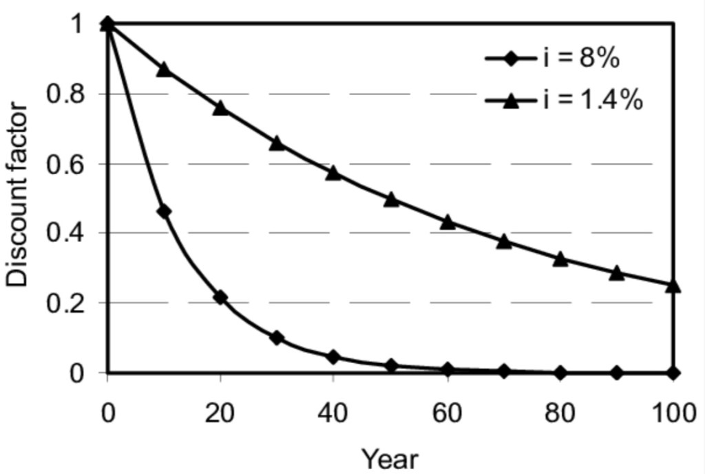
The new baseline discount rate proposed by OMB is 1.7%, and it is lower still for very distant flows of benefits. This is intended as a real, after-tax discount rate on Treasury bonds. It represents an average (and ex post) risk-free rate on bonds held to maturity over the historical period in question, calculated as described by OMB. However, like the earlier guidance, it is not prospective in any sense. And of course it is quite low!
Our Poor Little Rich Ancestors
The projected benefits of regulations or other public initiatives can be highly dubious in the first place. Unintended consequences are the rule rather than the exception. Furthermore, even modest economic growth over several generations will leave our ancestors with far more income and wealth than we have at our disposal today. That means their ability to adapt to changes will be far superior, and they will have access to technologies making our current efforts seem quaint.
Now here’s the thing: discounting the presumed benefits of government intervention at a low rate would drastically inflate their present value. John Cochrane uses an extreme case to illustrate the point. Suppose a climate policy is projected to avoid costs equivalent to 5% of GDP 100 years from now. Those avoided costs would represent a gigantic sum! By then, at just 2% growth, real GDP will be over seven times larger than this year’s output. Cochrane calculates that 5% of real GDP in 2123 is equivalent to 37% of 2023 real GDP. And the presumed cost saving goes on forever.
We can calculate the present value of the climate policy’s benefits to determine whether it’s greater than the proposed cost of the policy. Let’s choose a fairly low discount rate like … oh, say zero. In that case, the present value is infinite, and it is infinite at any discount rate below 2% (such as 1.7%). That’s because the benefits grow at 2% (like real GDP) and go on forever! That’s faster than the diminishing effect of discounting on present value. In mathematical terms, the series does not converge. Of course, this is not discounting. It is non-discounting. Cochrane’s point, however, is that if you take these calculations seriously, you’d be crazy not to implement the policy at any finite cost! You shouldn’t mind the new taxes at all! Or the inflation tax induced by more deficit spending! Or higher regulatory costs passed along to you as a consumer! So just stop your bitching!
Formal Comments to OMB
If Cochrane’s example isn’t enough to convince you of the boneheadedness of the OMB proposal, there are several theoretical reasons to balk. Cochrane provides links to a couple of formal comments submitted to OMB. Joshua Rauh of the Stanford Business School details a few fundamental objections. His first point is that a regulatory impact analysis (RIA), or the evaluation of any other initiative, “should be based on market conditions that prevail at the time of the RIA”. In other words, the choice of a discount rate should not rely on an average over a lengthy historical period. Second, it is unrealistic to assume that the benefits and costs of proposed regulations are risk-free. In fact, unlike Treasury securities, these future streams are quite risky, and they are not tradable, and they are not liquid.
Rauh also notes that the OMB’s proposed decline in discount rates to be applied to benefits or cash flows in more distant periods has no reliable empirical basis. He believes that results based on a constant discount rate should at least be reported. Moreover, agencies should be required to offer justification for their choice of a discount rate relative to the risks inherent in the streams of costs and benefits on any new project or rule.
Rauh is skeptical of recommendations that agencies should add a theoretical risk premium to a risk-free rate, however, despite the analytical superiority of that approach. Instead, he endorses the simplicity of the OMB’s previous guidance for discount rates of 3% and 7%. But he also proposes that RIAs should always include “the complete undiscounted streams of both benefits and costs…”. If there are distributions of possible cost and benefit streams, then multiple streams should be included.
Furthermore, Rauh says that agencies should not recast streams of benefits in the form of certainty equivalents, which interpose various forms of objective functions in order to calculate a “fair guarantee”, rather than a range of actual outcomes. Instead, Rauh insists that straightforward expected values should be used, This is for the sake of transparency and to enable independent assessment of RIAs.
Another comment on the OMB proposal comes from a group of economists at MIT. They have fewer qualms than Rauh regarding the use of risk-adjusted discount rates by government agencies. In addition, they note that risk in the private sector can often be ameliorated by diversification, whereas risks inherent in public policy must be absorbed by changes in taxes, government spending, or unintended costs inflicted on the private sector. Taxpayers, those having stakes in other programs, and the general public bear these risks. Using Treasury rates for discounting presumes that bad outcomes have no cost to society!
Conclusion
Discounting the costs and benefits of proposed regulations and other government programs should be performed with discount rates that reflect risks. Treasury rates are wholly inappropriate as they are essentially risk-free over time horizons often much shorter than the streams of benefits and costs to be discounted. The OMB proposal might be a case of simple thoughtlessness, but I doubt it. To my mind, it aligns a little too neatly with the often expansive agenda of the administrative state. It would add to what is already a strong bias in favor of regulatory action and government absorption of resources. Champions of government intervention are prone to exaggerate the flow of benefits from their pet projects, and low discount rates exaggerate the political advantages they seek. That bias comes at the expense of the private sector and economic growth, where inter-temporal tradeoffs and risks are exploited only at more rational discounts and then tested by markets.
Government budget negotiations never fail to frustrate anyone of a small-government persuasion. We have a huge, ongoing federal budget deficit. Spending’s gone bat-shit out of control over the past several years and too few in Congress are willing to do anything about it. Democrats would rather see politically-targeted tax increases. While some Republicans advocate spending cuts, the focus is almost entirely on discretionary spending. Meanwhile, the entitlement state is off the table, including Social Security reform.
Fiscal Indiscretion
Sadly, non-discretionary outlays (entitlements) today make a much larger contribution to the deficit than discretionary spending. That includes the programs like Social Security (SS) and Medicare, in which spending levels are programmatic and not subject to annual appropriations by Congress. When these programs were instituted there were a large number of workers relative to retirees, so tax contributions exceeded benefit levels for many decades. The revenue excesses were placed into “trust funds” and invested in Treasury debt. In other words, surpluses under non-discretionary SS and Medicare programs were used to finance discretionary spending!
The aging of Baby Boomers ultimately led to a reversal in the condition of the trust funds. Fewer workers relative to retirees meant that annual payroll tax collections were not adequate to cover annual benefits, and that meant drawing down the trust funds. Current projections by the system trustees call for the SS Trust Fund to be exhausted by 2035. Once that occurs, benefits will automatically be reduced by roughly 20% unless Congress acts to shore up the system before then.
A Few Proposals
I’ve written about the need for SS reform on several occasions (though the first article at that link is not germane here). It seems imperative for Congress and the President to address these shortfalls. By all appearances, however, many Republicans have put the issue aside. For his part, Joe Biden has apparently accepted the prospect of an automatic reduction in benefits in 2035, or at least he’s willing to kick that can down the road. He has, however, endorsed taxes on high earners to fund Medicare. Senator John Kennedy (R-LA) suggests raising the retirement age, or at least raise the minimum age at which one may claim benefits (now 62). Senators Bill Cassidy (R-La.) and Angus King (I-Maine) were working on a compromise that would create an investment fund to fortify the system, but the specifics are unclear, as well as how much that would accomplish.
Meanwhile, Senator Bernie Sanders (S-VT) proposes to expand SS benefits by $2,400 a year and add funding by extending payroll taxes to earners above the current limit of $160,000. Senator Joe Manchin (D-WV) has endorsed the latter as a “quick fix”.
There is also at least oneproposal in Congress to end the practice of taxing a portion of SS benefits as income. I have trouble believing it will gain wide support, despite the clear double-taxation involved.
Then there are always discussions of reducing benefits at higher income levels or even means-testing benefits. In fact, it would be interesting to know what proportion of current benefits actually function as social insurance, as opposed to a universal entitlement. The answer, at least, could serve as a baseline for more fundamental reforms, including changes in the structure of payroll taxes, voluntary lump-sum payouts, and private accounts.
More Radical Views
There are a few prominent voices who claim that SS is sustainable in its current form, but perhaps with a few “no big deal” tax increases. Oh, that’s only about a $1 trillion “deal”, at least for both Medicare and SS. More offensive still are the scare tactics used by opponents of SS reform any time the subject comes up. I’m not aware of any serious reform proposal made over the past two decades that would have affected the benefits of anyone over the age of 55, and certainly no one then-eligible for benefits. Yet that charge is always made: they want to cut your SS benefits! The Democrats made that claim against George W. Bush, torpedoing what might have been a great accomplishment for all. And now, apparently Donald Trump is willing to use such accusations to damage any rival who has ever mentioned reform, including Mike Pence. Will you please cut the crap?
The System
The thing to remember about SS is that it is currently structured as a pay-as-you-go (PAYGO) system, despite the fact that benefits are defined like many creaky private pensions of old. SS benefits in each period are paid out of current “contributions” (i.e., FICO payroll taxes) plus redemptions of government bonds held in the Trust Fund. Contributions today are not “invested” anywhere because they are not enough to pay for current benefits under PAYGO.
The Trust Fund was accumulated during the years when favorable demographics led to greater FICO contributions than benefit payouts. The excess revenue was “invested” in Treasury bonds, which meant it was used to fund deficits in the general budget. It’s been about 15 years since the Trust Fund entered a “draw-down” status, and again, it will be exhausted by 2035.
SSA Says It’s a Good Deal
A participant’s expected “rate of return” on lifetime payroll tax payments depends on several things: lifetime earnings, age at which benefits are first claimed, life expectancy at that time, marital status, relative earning levels within two-earner couples, and the “full retirement age” for the individual’s birth year. Payroll tax payments, by the way, include the employer’s share because that is one of the terms of a hire. A high rate of return is not the same as a high level of benefits, however. In fact, relative to career income, SS has a great deal of progressivity in terms of rates of return, but not much in terms of benefit levels.
The Social Security Administration (SSA) has calculated illustrative real internal rates of return (IRR) for many categories of earners given certain assumptions. (An IRR is a discount rate that equalizes the present value (PV) of a stream of payments and the PV of a stream of payoffs.) The SSA’s most recent update of this exercise was in April 2022. The report references Old Age, Survivors, and Disability Insurance (OASDI), but the focus is exclusively on seniors.
Three basic scenarios were considered: 1) current law, as scheduled, despite its unsustainability; 2) a payroll tax increase from 12.4% (not including the Medicare tax) to 15.96% starting in 2035, when the Trust Fund is exhausted; and 3) a reduction in benefits of 22% starting in 2035.
The authors of the report concludethat “… the real value of OASDI benefits is extraordinarily high.” This theme has been echoed by several other writers, such as here and here. This conclusion is based on a comparison to returns earned by investments that SSA judges to have comparably low risk.
I note here that I’ve made assertions in the past about relative SS returns based on nominal benefits, rather than inflation-adjusted values. Those comparisons to private returns might have seemed drastic because they were expressed in terms of hypothetical future nominal values at the point of retirement. The gaps are not as large in real terms or if we consider SS returns broadly to include those accruing to low career earners. Medium and high earners tend to earn lower hypothetical returns from SS.
A Mixed Bag
SSA’s calculated IRRs are highest for one-earner couples followed by two-earner couples. Single males do relatively poorly due to their higher mortality rates. Low earners do very well relative to higher earners. Earlier birth years are associated with higher IRRs, but these are not as impressive for cohorts who have not yet claimed benefits. The ranges of birth years provided in the report make this a little imprecise, but I’ll focus on those born in 1955 and later.
Of course the returns are highest under the current law hypothetical than for the scenarios involving a benefit reduction or a payroll tax hike. The current law IRRs can be viewed as baselines for other calculations, but otherwise they are irrelevant. The system is technically insolvent and the scheduled benefits under current law can’t be maintained beyond 2034 without steps to generate more revenue or cut benefits. Those steps will reduce IRRs earned by hypothetical SS “assets” whether they take the form of higher payroll taxes, lower benefits, a greater full retirement age, or other measures.
The tax hike doesn’t have much impact on the IRRs of near-term retirees. It falls instead on younger cohorts with some years of employment (and payroll tax payments) remaining. The effect of a cut in benefits is spread more evenly across age cohorts and the reductions in IRRs is somewhat larger.
With higher payroll taxes after 2034, the average IRRs for birth years of 1955+ range from about 0.5% up to about 6.25%. The returns for single females and two-earner couples are roughly similar and fall between those for single males on the low end and one-earner couples on the high end. In all cases, low earners have much higher IRRs than others.
The reduction in benefits produces returns for the 1955+ age cohorts averaging small, negative values for high-earning single men up to 5.5% to 6% for low-earning, one-earner couples.
But On the Whole…
The IRR values reported by SSA are quite variable across cohorts. Individuals or couples with low earnings can usually expect to “earn” real IRRs on their contributions of better than 3% (and above 5% in a few cases). Medium earners can expect real returns from 1% to 3% (and in some cases above 4%). Many of the returns are quite good for a safe “asset”, but not for high earners.
Again, SSA states that these are real returns, though they provide no detail on the ways in which they adjust the components used in their IRR formula to arrive at real returns. Granting the benefit of the doubt, we saw persistently negative real returns on a range of safe assets in the not-very-distant past, so the IRRs are respectable by comparison.
Qualifications
There are many assumptions in the SSA’s analysis that might be construed as drastic simplifications, such as no divorce and remarriage, uniform career duration, and no relationship between earnings and mortality. But it’s easy to be picky. Many of the assumptions discernible from the report seem to be reasonable simplifications in what could otherwise be an unruly analysis. Nonetheless, there are a few assumptions that I believe bias the IRRs upward (and perhaps a few in the other direction).
In fact, SSA is remarkably non-transparent in their explanation of the details. Repeated checking of SSA’s document for clear answers is mostly futile. Be that as it may, I’m forced to give SSA the benefit of the doubt in several respects. One is the reinvestment of cumulative remaining contributions at the IRR throughout the earning career and retirement. A detailed formula with all components and time subscripts would have been nice.
… And Major Doubts
As to my misgivings, first, the IRRs reported by SSA are based on earners who all reach the age of 65. However, roughly 14% – 15% of individuals who live to be of working age die before they reach the age of 65. Most of those deaths occur in the latter part of that range, after many years of contributions and hypothetical compounding. That means the dollar impact of contributions forfeited at death before age 65 is probably larger than the unweighted share of individuals. These individuals pay-in but receive no retirement benefit in SSA’s IRR framework, although some receive disability benefits for a period of time prior to death. It wouldn’t bother my conscience to knock off at least a tenth of the quoted returns for this consideration alone.
A second major concern surrounds the method of calculating benefits and discounted benefits. SSA assumes that benefits continue for the expected life of the claimant as of age 65. If life expectancy is 19 years at age 65, then “expected” benefits are a flat stream of benefit payments for 19 years. Discounting each payment back to age 65 at the IRR yields one side of the present value equality. This constant cash flow (CCF) treatment is likely to overstate the present value of benefits. Instead of CCFs, each payment should be weighted by the probability that the claimant will be alive to receive it with a limit at some advanced age like 100. CCF overcounts present values up to the expected life, but it undercounts present values beyond the expected life because the assumed CCF benefits then are zero!! Weighting benefit payments by the probability of survival to each age produces continuing additions to the PV, but increasing mortality and decaying discount factors become quite substantial beyond expected life, leading to relatively minor additions to PV over that range. The upshot is that the CCFs employed by SSA overstate PVs by front-loading all benefits earlier in retirement. For a given PV of contributions, an overstated PV of benefits requires a higher (and overstated) IRR to restore the PV equality, and this might be a substantial source of upward bias in SSA’s calculations.
Third, when comparing an SS “asset” to private returns, a big difference is that private balances remaining at death become assets of the earner’s estate. Meanwhile, a single beneficiary forfeits their SS benefits at death (except for a small death benefit), while a surviving spouse having lower benefits receives ongoing payments of the decedent’s benefits for life. This consideration, however, in and of itself, means that private plans have a substantial advantage: the “expected” residual at death can be “optimized” at zero or some higher balance, depending on the strength of the earner’s bequest motive.
Finally, in a footnote, the SSA report notes that their treatment of income taxes on Social Security benefits for claimants with higher incomes might bias some of the IRRs upward. That seems quite likely.
It would be difficult to recast SSA’s report based on adjustments for all of these qualifications. However, it’s likely that the IRRs in the SSA report are sharply overstated. That means many more beneficiaries with medium and higher earnings records would have returns in the 0% to 2% range, with more IRRs in the negative range for singles. Low earners, however, might still get returns in a range of 3% to 5%.
The SSA analysis attempts to demonstrate some limits to the risks faced by participants, given the scenarios involving a payroll tax increase or a benefits reduction in 2035. Nevertheless, there are additional political risks to the returns of certain classes of current and future retirees. For example, payroll taxes could be made much more progressive, benefits could be made subject to means testing, or indexing of benefits could be reduced. In fact, there are additional demographic risks that might confront retirees several decades ahead. Continued declines in fertility could further undermine the system’s solvency, requiring more drastic steps to shore up the system. As a hypothetical asset, by no means is SS “risk-free”.
Better Returns
Now let’s consider returns earned by private assets, which represent investments in productive capital. For stocks, these include the sum of all dividends and capital gains (growth in value). For compounding purposes, we assume that all returns are reinvested until retirement. Remember that private returns are much less variable over spans of decades than over durations of a few years. Over the course of 40 year spans (SSA’s career assumption), private returns have been fairly stable historically, and have been high enough to cushion investors from setbacks. Here is Seeking Alpha on annualized returns on the basket of stocks in the S&P 500:
“… the return on the S&P 500 since the beginning of valuation in 1928, is 10.22%, whereas the inflation-adjusted return on the market since that time is 7.01%…”
That real return would generate benefits far in excess of SS for most participants, but it’s not an adequate historical perspective on market performance. A more complete picture of real returns on the S&P, though one that is still potentially flawed, emerges from this calculator, which relies on data from Robert Shiller. The returns extend back to 1871, but the index as we know it today has existed only since 1957. The earlier returns tend to be lower, so these values may be biased:
Real stock market returns over rolling 40-year time spans varied considerably over this longer period. Still, those kind of stock returns would be superior to the IRRs in the SSA report going forward in all but a few cases (and then only for low and very low earners).
Most workers facing a choice between investing at these rates for 40 years, with market risk, and accepting standard SS benefits, uncertain as they are, couldn’t be blamed for choosing stocks. In fact, if we think of contributions to either type of plan as compounding to a hypothetical sum at retirement, the stock investments would produce a “pot of gold” several times greater in magnitude than SS.
However, we still don’t have a fair comparison because workers choosing a stock plan would essentially engage in a kind of dollar-cost averaging over 40 years, meaning that investments would be made in relatively small amounts over time, rather than investing a lump-sum at the beginning. This helps to smooth returns because purchases are made throughout the range of market prices over time, but it also means that returns tend to be lower than the 40-year rolling returns shown above. That’s because the average contribution is invested for only half the time.
To be very conservative, if we assume that real stock returns average between 5% and 6% annually, $1 invested every year would grow to between $131 – $155 after 40 years in constant dollars. At returns of 1% to 2% from SS, which I believe are typical of the IRRs for many medium earners, the cumulative “pot” would grow to $49 – $60. Assuming that the tax treatment of the stock plan was the same as contributions and benefits under SS, the stock plan almost triples your money.
Dealing With the Transition
Privatization covers a range of possible alternatives, all of which would require federal borrowing to pay transition costs. Unfortunately, the Achilles heel in all this is that now is a bad time to propose more federal borrowing, even if it has clear long-term benefits to future retirees.
Todd Henderson in the Wall Street Journal suggests a seeding of capital provided by government at birth along with an insurance program to smooth returns. Another idea is to offer an inducement to delay retirement claims by allowing at least a portion of future benefits to be taken as a lump sum. If retirees can privately invest at a more advantageous return, they might be willing to accept a substantial discount on the actuarial value of their benefits.
In fact, there is evidence that a majority of participants seem to prefer distributions of lump sums because they don’t value their future benefits at anything like that suggested by the SSA analysis. In fact, many participants would defer retirement by 1 – 2 years given a lump sum payment. Discounts and/or delayed claims would reduce the ultimate funding shortfall, but it would require substantial federal borrowing up front.
Additional federal borrowing would also be required under a private option for investing one’s own contributions for future dispersal. The impact of this change on the system’s long-term imbalances would depend on the share of earners willing to opt-out of the traditional SS program in whole or in part. More opt-outs would mean a smaller long-term obligations for the traditional system, but it would be hampered by a costly transition over a number of years. Starting from today’s PAYGO system, someone still has to pay the benefits of current retirees. This would almost certainly mean federal borrowing. Spreading the transition over a lengthy period of time would reduce the impact on credit markets, but the borrowing would still be substantial.
For example, perhaps earners under 35 years of age could begin opting out of a portion or all of the traditional program at their discretion, investing contributions for their own future use. Thus, only a small portion of contributions would be diverted in the beginning, and amounts diverted would contribute to the nation’s available pool of saving, helping to keep borrowing costs in check. By the time these younger earners reach retirement age, nearly all of today’s retirees will have passed on. Ultimately, the average retiree will benefit from higher returns than under the traditional program, but since they won’t be (fully) paying the benefits of current or near-term retirees, the public must come to grips with the bad promises of the past and fund those obligations in some other way: reduced benefits, taxes, or borrowing.
Another objection to privatization is financial risk, particularly for lower-income beneficiaries. Limiting opt-outs to younger earners with adequate time for growth would mitigate this risk, along with a reversion to the traditional program after age 45, for example. Some have proposed limiting opt-outs to higher earners. Bear in mind, however, that the financial risk of private accounts should be weighed against the political and demographic risk already inherent in the existing system.
One more possibility for bridging the transition to private, individually-controlled accounts is to sell federal assets. I have discussed this before in the context of funding a universal basic income (which I oppose). The proceeds of such sales could be used to pay the benefits of current and near-term retirees so as to allow the opt-out for younger workers. Or it could be used to pay off federal debt accumulated in the process. The asset sales would have to proceed at a careful and deliberate pace, perhaps stretching over several decades, but those sales could include everything from the huge number of unoccupied federal buildings to vast tracts of public lands in the west, student loans, oil and gas reserves, and airports and infrastructure such as interstate highways and bridges. Of course, these assets would be more productive in private hands anyway.
The Likely Outcome
Will any such privatization plan ever see the light of day? Probably not, and it’s hard to guess when anything will be done in Washington to address the insolvency we already face. Instead, we’ll see some combination of higher payroll taxes, higher payroll taxes on high earners through graduated payroll tax rates or by lifting the earnings cap, reduced benefits on further retirees, limits on COLAs to low career earners, and means-tested benefits. Some have mentioned funding Social Security shortfalls with income taxes. All of these proposals, with the exception of automatic benefit cuts in 2035, would require acts of Congress.
In advanced civilizations the period loosely called Alexandrian is usually associated with flexible morals, perfunctory religion, populist standards and cosmopolitan tastes, feminism, exotic cults, and the rapid turnover of high and low fads---in short, a falling away (which is all that decadence means) from the strictness of traditional rules, embodied in character and inforced from within. -- Jacques Barzun